Performance of Arbitrary-Precision Numerical Libraries

(last update: September 17, 2026)

Summary

For computations that need linear algebra and FFTs at 100–1000 decimal digits (quantum-mechanical calculations in my case), I measured the speed of the major arbitrary-precision libraries and systems under identical conditions. This is a sequel to my 2020 Qiita article (in Japanese). The scope is now (A) scalar arithmetic, (B) diagonalization of nonsymmetric and Hermitian matrices, and (C) complex FFTs, and the article also covers the effect of parallelization and estimates of the actual computing resources (time and memory) required.

The conclusions first:

1. Sequential (single-threaded) arbitrary-precision diagonalization falls within a factor of about 2 regardless of language or library. Speed is set by the cost of arbitrary-precision scalar operations; the quality of the implementation contributes only a factor of about 2.

2. The way out is parallelization, and among the candidates tested only Advanpix parallelizes the eigenvalue routines themselves. On 64 physical cores, nonsymmetric diagonalization at \(d=1000\) digits and matrix size \(N=300\) runs 19× faster than on one thread, and 20–60× faster than the sequential group. SMT (128 threads), however, is counterproductive; the thread count must be pinned to the number of physical cores.

3. MPLAPACK's OpenMP BLAS (Rgemm) scales well, 56× on 64 cores, but more than 90% of the eigenvalue routines (Rgeev/Cheev) is spent in QR iteration and eigenvector computation (level 1 and 2 operations), so the parallel BLAS yields only a 1.1× gain.

4. For scalar arithmetic, arb's transcendental functions are 4–6× faster than MPFR's, and the transcendental functions of Boost.Multiprecision's cpp_bin_float are unusable. If fixed precision suffices, MultiFloats (Float64x2/x4) is faster than dd/qd and __float128.

5. For FFTs of power-of-two length, a simple OpenMP implementation is fast enough (\(2^{20}\) points at 1000 digits in 1 second on 128 threads). For composite lengths Advanpix is the only practical option; FLINT becomes 50× slower than at \(2^{20}\).

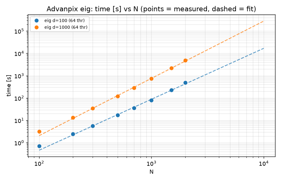
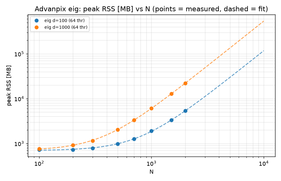
6. The resources needed by Advanpix (64 threads) can be estimated as time \(t \approx 6\times10^{-7}\,(d/1000)\,N^3\) seconds (conservative) and memory \(M \approx 0.7\ \mathrm{GB} + N^2\,(700 + 4.7\,d)\) bytes, where \(d\) is the number of digits. Diagonalizing \(N=10000\) at 1000 digits needs 525 GB of memory; memory becomes the limiting factor before time does.

About the writing of this article

This article was produced with Anthropic's Claude (Fable 5.1, reasoning level: medium). The evaluation plan was drafted by Claude, based on the previous evaluation, with the goal of being as fair as possible. The benchmark code for each language, the aggregation and fitting scripts, the interpretation of the results, and the draft of this text were produced interactively; running the measurements, checking the results, and configuring the environment were all done by a human. Responsibility for the content lies with the author (in princicple. I honestly has hard to keep up with one :-< ).

I have also come to appreciate how mature the numerical libraries for arbitrary precision and interval arithmetic have become, and I thank the maintainers who develop them. This article is only an evaluation, as of September 17, 2026, of the part of my own research that is the computational bottleneck; with generative AI, the code of each library will presumably improve further.

1. Environment and design of the measurements

Machine

Item	Content
CPU	AMD Ryzen Threadripper PRO 3995WX (64 cores / 128 threads, Zen 2, 1 NUMA node)
Memory	DDR4, 8 channels, 512 GB (ECC)
OS / compiler	Debian sid, gcc 16.2, -O2 -march=native
Libraries	GMP 6.3, MPFR 4.2.2, FLINT 3.6.0 (with arb merged in), MPLAPACK 3.0.0, Eigen 3.4 + mpreal, Boost.Multiprecision, QD 2.3
Language systems	Julia 1.13 (GenericSchur, GenericLinearAlgebra, MultiFloats 3.3, Arblib 1.8, GenericFFT), Python 3.14 (mpmath 1.3 + gmpy2, python-flint), MATLAB R2026a + Advanpix MCT 5.4.8, Mathematica 15.0

The CPU frequency governor was pinned to performance, and no other jobs ran during the measurements. OpenMP threads were pinned to cores with OMP_PROC_BIND=true OMP_PLACES=cores. Each point is the median of 3 trials (1 trial for large \(N\)). The variation between trials was 0.1–1%, smaller than the markers in the figures.

Tasks

(A) Scalar arithmetic: add / mul / div / sqrt / exp / log / sin / dot (inner product) applied repeatedly to arrays \(x\), \(y\) of length \(10^5\); the time per operation is recorded in ns. gemm is the time in seconds of one real dense matrix product with \(N=100\).

(B) Diagonalization: the nonsymmetric matrix is the same Circus matrix as last time (\(A_{i,i}=1,\ A_{i+1,i}=-1,\ A_{i,i+k}=k+1\ (k=1,\dots,4)\)); the Hermitian matrix is a complex matrix whose upper triangle is generated from a common random sequence. \(N = 10\)–\(1000\). The call measured computes both eigenvalues and right eigenvectors (the equivalent of MATLAB's [V,D]=eig(A)). As checks, \(|\sum_k \lambda_k - \mathrm{tr}\,A|\) and the residual \(\max_k \|Av_k-\lambda_k v_k\|_\infty/(\|A\|_\infty\|v_k\|_\infty)\) were verified for every system (Appendix A).

(C) FFT: time of one forward transform of complex length \(n = 2^{12}, 2^{16}, 2^{20}, 10^6\) (composite \(= 2^6\cdot5^6\)). Checked by the round-trip error.

Precision: 100 digits (334 bits) and 1000 digits (3323 bits). Fixed-precision types (double-double = 32 digits, quad-double = 64 digits, binary128 = 34 digits) are shown separately at their effective number of digits.

Random numbers: every language uses the same xorshift64 sequence, so the same matrices and arrays are processed everywhere.

Two pitfalls

Two things I noticed only after starting the measurements are worth stating first; both affect the interpretation of the results.

The first is the mantissa length of the input. When a random number generated in double precision is converted to an arbitrary-precision type, the mantissa has 53 bits and the rest is zero. arb operates on the actual length of the mantissa, so with such input a 1000-digit multiplication finishes in 10 ns, and MPFR also skips trailing zero limbs in multiplication and appears about 6× faster than it is. Here the inputs are sqrt(u), which fills the mantissa to the target precision. Be wary of benchmarks that use "values converted from double precision".

The second is that the Circus matrix is already upper Hessenberg (lower bandwidth 1). A general eigenvalue computation has three stages, Hessenberg reduction → QR iteration → eigenvector computation, and for the Circus matrix the first stage is trivial. So the diagonalization benchmarks, both last time and this time, measure the speed of "QR iteration and eigenvector computation" and do not reflect the performance of the Hessenberg reduction, which contains BLAS3 and is the easiest part to parallelize. The effect of this is examined separately with dense matrices in Section 5.

All code and raw measurements (CSV) are published (Appendix C).

2. Scalar arithmetic

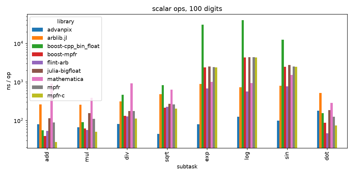
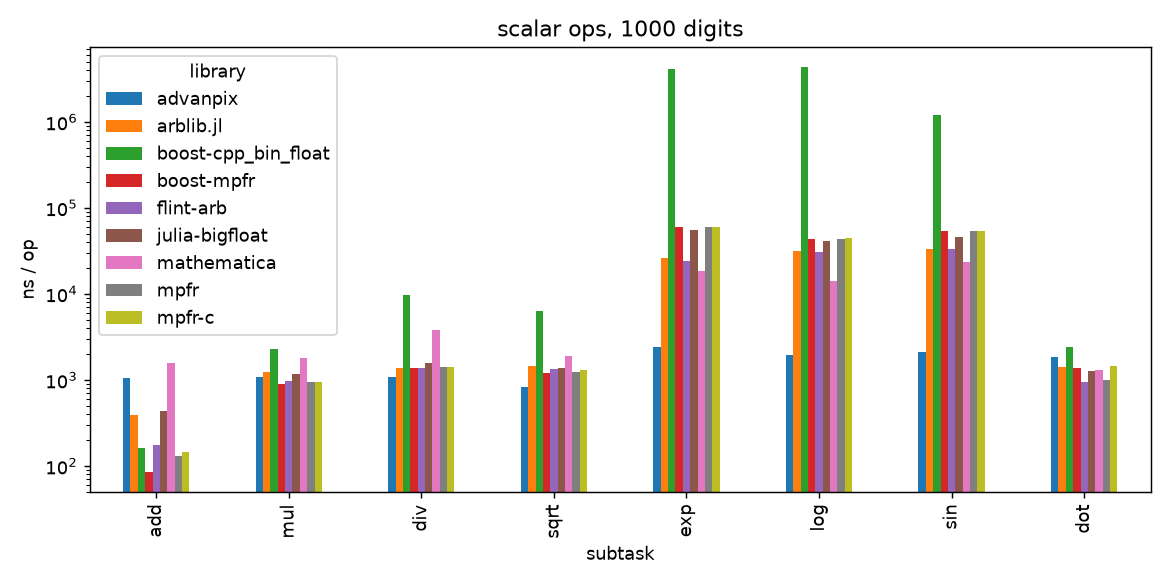
Time per operation at 100 digits (ns). add/mul/div/sqrt/exp/log/sin are per array element; gemm is converted to the time in seconds of one \(N=100\) matrix product.

System	add	mul	div	sqrt	exp	log	sin	dot	gemm N=100 [s]
MPFR C API (preallocated)	28	51	113	202	2360	4340	2460	74	0.081
Boost.Multiprecision mpfr_float	40	63	131	215	2400	4330	2470	87	0.087
mpreal (C++ wrapper)	88	111	175	264	2450	4410	2510	124	0.124
Julia BigFloat	114	155	175	273	2520	4430	2760	186	0.127
FLINT arb (C API)	54	57	128	226	678	564	769	46	—
Arblib.jl	263	255	313	481	887	725	797	515	0.288
Boost cpp_bin_float	56	91	462	822	30700	39800	12500	156	0.156
Mathematica	901	387	925	634	1010	939	1520	287	0.270
Advanpix (64-thread array operations)	79	67	81	45	79	126	100	179	0.003

The baseline is the raw MPFR C API: add 28 ns, mul 51 ns. The thinness of the wrapper shows directly: Boost's mpfr_float costs +40%, mpreal 3×, Julia's BigFloat 4×. The latter two create and destroy objects (malloc) on every operation; in Julia every BigFloat operation allocates on the heap.

Transcendental functions look different. arb's exp/log/sin (680 / 560 / 770 ns) are 4–6× faster than MPFR's (2.4 / 4.3 / 2.5 µs). arb has its own algorithms (piecewise polynomial approximation and the bit-burst method), which is a reason to choose arb for computations that call transcendental functions heavily at high precision. Boost's cpp_bin_float is more than 10× slower than MPFR for transcendental functions (exp takes 4 ms at 1000 digits) and should not be used at 100 digits or more.

Advanpix executes array operations on 64 threads, so this table shows "64-thread array operations divided by the number of elements". It dominates for heavy operations — exp at 79 ns, gemm at 3 ms — but is slower than MPFR for light operations such as add (79 ns, 1 µs at 1000 digits), because the thread start-up and memory-bandwidth overheads are not hidden by light operations. The picture is "heavy operations: Advanpix; large loops of light operations: not suited".

At 1000 digits, multiplication converges to about 950 ns in every system. They all share GMP's multiplication kernel, so wrapper differences vanish in this regime. A notable point is Mathematica: its transcendental functions are among the slowest at 100 digits (1 µs) but 3× faster than MPFR at 1000 digits (exp 18 µs vs 60 µs); its high-precision algorithms are well done.

Fixed-precision types (effective 32–64 digits) form a separate table.

Type	Digits	add	mul	div	sqrt	exp	log	sin
MultiFloats Float64x2	32	1.4	0.9	1.3	1.7	122	37	2670*
QD dd_real	32	1.2	2.9	7.9	10.5	232	261	232
DoubleFloats Double64	32	7.6	7.4	7.8	3.4	71	62	150
__float128	34	20.5	18.9	32	406	646	652	533
MultiFloats Float64x4	64	7.0	7.1	23	42	903	1300	3590*
QD qd_real	64	20	37	202	602	2330	7320	2120

(* sin in MultiFloats falls back to BigFloat)

Float64x2 matches or beats dd_real with add 1.4 ns and mul 0.9 ns, and Float64x4 is 3–5× faster than qd_real. MultiFloats benefits from being a Julia type that vectorizes with SIMD. __float128 takes 20 ns, 15× slower than Float64x2 at almost the same precision (34 vs 32 digits), so on x86, which has no hardware support for it, double-double is the better deal.

3. Diagonalization — sequential performance

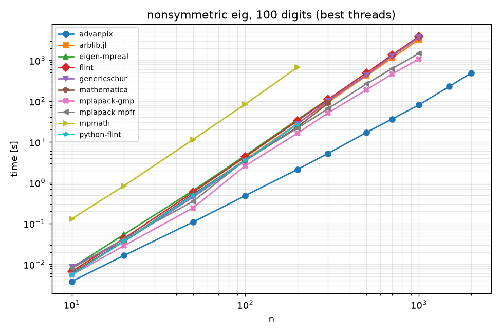
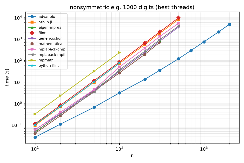
First, the single-threaded comparison. Time in seconds for the nonsymmetric (Circus) matrix at \(N=300\).

System	100 digits	1000 digits	Arithmetic
Advanpix	34.9	653	real
MPLAPACK Rgeev (GMP mpf)	51.4	1310	real
MPLAPACK Rgeev (MPFR)	71.0	971	real
Mathematica Eigensystem	89.1	700	real
Arblib.jl approx_eig_qr	93.8	1850	complex
Julia GenericSchur	103	794	real
Eigen EigenSolver + mpreal	112	790	real
FLINT acb_mat_approx_eig_qr	113	2170	complex
python-flint	(N=200: 27.3)	—	complex
mpmath	(N=200: 678)	—	real

The systems fall into two groups. Those that solve with real Hessenberg QR (Advanpix, MPLAPACK, Mathematica, GenericSchur, Eigen) sit together at 650–970 s for 1000 digits, and those that solve in complex arithmetic (FLINT, Arblib) are 2–3× slower. The eigenvalues of the Circus matrix are complex but the matrix is real, so implementations that go through the real Schur form avoid complex multiplications (4 real multiplications each). The remaining differences are implementation quality and lie within a factor of 1.5.

Mathematica, which looked slow in the previous article, is in the fastest class as long as the arbitrary-precision Eigensystem is used sequentially (700 s at 1000 digits, \(N=300\), faster than GenericSchur and Eigen). The earlier impression came from comparing it with the parallelized Advanpix. mpmath is an order of magnitude slower (678 s at 100 digits, \(N=200\), versus 20–35 s for the others); from Python, python-flint (as fast as FLINT in C) is the one to use.

The differences widen with \(N\). Going from \(N=300\) to \(1000\) at 100 digits, MPLAPACK goes from 71 to 1470 s (20.7×, \(\approx N^{2.5}\)), while GenericSchur goes from 103 to 3610 s and Arblib from 94 to 3240 s (35×, \(\approx N^{3.0}\)); at \(N=1000\) MPLAPACK is 2.5× faster than GenericSchur. This is presumably the regime in which the LAPACK-derived blocking pays off in cache efficiency. At 1000 digits the cost of a single operation dominates and this difference disappears (at \(N=500\): GenericSchur 3580 s, MPLAPACK 3980 s).

MPLAPACK's backend is best chosen by precision. At 100 digits GMP's mpf, which is lighter because it does not do correct rounding, is 1.3–1.5× faster than MPFR; at 1000 digits MPFR's multiplication optimizations win and it is 1.4× faster.

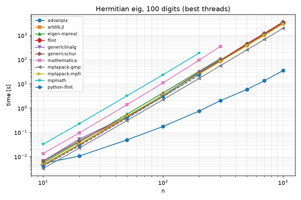
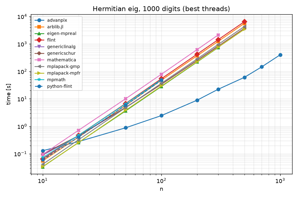
Hermitian matrix (\(N=300\), 1 thread, seconds).

System	100 digits	1000 digits	Solver
Advanpix	18.2	246	dedicated (auto-detected)
MPLAPACK Cheev (GMP)	55.2	951	dedicated
MPLAPACK Cheev (MPFR)	82.2	749	dedicated
Arblib.jl	89.6	1230	general
FLINT	89.9	1420	general
GenericSchur eigen(Hermitian)	93.4	821	dedicated
GenericLinearAlgebra	103	841	dedicated
Eigen SelfAdjointEigenSolver	109	736	dedicated
Mathematica	347	2110	dedicated (auto-detected)

Surprisingly, there is almost no difference between the dedicated Hermitian solvers (tridiagonalization + QR) and FLINT's general solver. In double precision a dedicated solver is several times faster than a general one, but in arbitrary precision the cost of scalar operations dominates and the difference in operation count (1/3–1/4 of the general solver) hardly shows in the time. Mathematica is last for Hermitian matrices. The same Mathematica solves the nonsymmetric Circus matrix in 700 s (1000 digits, \(N=300\)) but takes 2110 s, 3× longer, for the Hermitian matrix. In every other system the Hermitian case is as fast as or faster than the nonsymmetric one, so only Mathematica is reversed. HermitianMatrixQ returns True, so the dedicated path should be taken, which means that path is slower than the general one. Advanpix is the only system in which the dedicated routine clearly pays off: even on one thread its Hermitian solve is 2.7× faster than its nonsymmetric one.

Certified eigenvalues (FLINT acb_mat_eig_multiple, which proves enclosures of the eigenvalues with interval arithmetic) work at 100 digits with an interval radius of \(10^{-56}\) at \(N=100\), but the radius grows to \(10^{-8}\) at \(N=200\) and the certification fails at \(N=300\). At 1000 digits it succeeds up to \(N=300\) but takes 3.3 hours (the approximate solution takes 36 minutes). The condition number of the eigenvectors of the Circus matrix deteriorates rapidly with \(N\), so certified computation is limited to \(N \le 100\) or to cases with a large precision margin.

Among fixed-precision types, MultiFloats' Float64x2 takes 2.8 s at \(N=300\) and Float64x4 24 s (35× faster than 100-digit BigFloat), and 101 s / 815 s even at \(N=1000\). If 32–64 digits suffice, there is no reason to use an arbitrary-precision type.

4. Diagonalization — parallelization

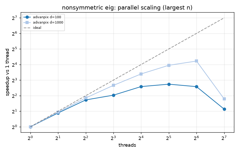
Advanpix time (seconds, \(N=300\)) as the thread count is varied from 1 to 128.

Threads	1	2	4	8	16	32	64	128
Nonsymmetric, 100 digits	34.9	18.9	10.5	8.5	5.8	5.2	5.8	15.9
Nonsymmetric, 1000 digits	653	339	180	103	62	42	35	189
Hermitian, 1000 digits	246	131	73	44	29	22	22	38

At 1000 digits the scaling is close to ideal up to the 64 physical cores, 18.7×; at 100 digits it stalls at 6.7× with 32 threads. With fewer digits the parallel granularity is too fine and the thread start-up overhead becomes relatively large. With 128 SMT (Simultaneous Multi-Threading, Hyper-Threading) threads the run becomes more than 5× slower; even at \(N=10\), 5 ms becomes 500 ms. When using Advanpix, pin maxNumCompThreads to the number of physical cores. Parallel efficiency also improves with \(N\): at 1000 digits the time from \(N=300\) to \(1000\) grows only 21× (equivalent to \(N^{2.5}\)).

No other system gets faster with more threads. MPLAPACK's OpenMP build (--enable-optimization) gives 1.04–1.08× for Rgeev/Cheev even at 8 threads and degrades at 128. FLINT's approx_eig_qr is independent of the thread count, and Julia's GenericSchur/Arblib are not parallelized. The "overwhelming" advantage of Advanpix seen in the previous article is parallelization: a difference of 1.2–3× on one thread becomes 20–60× on 64 threads.

5. Where MPLAPACK's parallelization takes effect

MPLAPACK is a port of the reference LAPACK to arbitrary-precision types, with OpenMP versions of some BLAS routines (Rgemm and others). To find out why this did not help the eigenvalue computation, I measured Rgemm, Rgehrd (Hessenberg reduction), and Rgeev (general eigenproblem) individually on a dense random matrix (sqrt input) and gave the same matrix to Advanpix.

Routine	Digits	N	1 thread	8	64	Speedup at 64
MPLAPACK Rgemm	100	1000	100 s	14.4	2.30	44
Advanpix gemm	100	1000	76.7	9.9	2.01	38
MPLAPACK Rgemm	1000	1000	977	125	17.4	56
Advanpix gemm	1000	1000	1260	166	27.1	46
MPLAPACK Rgehrd	100	1000	199	72	59	3.4
MPLAPACK Rgehrd	1000	1000	1671	587	461	3.6
MPLAPACK Rgeev (dense)	100	300	57.1	49.1	49.5	1.16
MPLAPACK Rgeev (dense)	1000	300	831	759	757	1.10
Advanpix eig (dense)	100	300	44.7	10.0	6.6	6.8
Advanpix eig (dense)	1000	300	756	117	39.5	19

Rgemm alone scales well, 44–56× on 64 cores, as the author claims; at 1000 digits it is 1.3–1.5× faster than Advanpix's matrix product. The Hessenberg reduction Rgehrd benefits from Rgemm in its blocked part, but the level 2 operations (gemv inside Rlahr2) remain, so it saturates at 3.5×. The double-precision dgehrd has the same structure.

The issue is the breakdown of Rgeev: for the dense matrix at \(N=300\) and 1000 digits, Rgehrd takes 46 s while the whole Rgeev takes 831 s. The Hessenberg reduction is only 5–10% of the total; the remaining 90% or more goes to QR iteration (Rhseqr) and eigenvector computation (Rtrevc). In the reference LAPACK these two are written with level 1 and 2 operations and never call BLAS3, so however fast the parallel BLAS is, Rgeev can gain at most 1.1×. The 1.04× on the Circus matrix was because the Hessenberg reduction was trivial there, and the dense case does not change the essence.

Double precision is no different: numpy's and Mathematica's double-precision eig appear to use several cores because the gemm in the underlying OpenBLAS / MKL is parallel. LAPACK itself is not parallelized. In double precision the parts that call gemm (zgehrd, zlaqr5, ztrevc3) make up a fair fraction and give a speedup of a few times, but in arbitrary precision the gemm calls are too fine-grained and even that effect vanishes.

Advanpix, by contrast, goes from 756 s on one thread (about the same as MPLAPACK's 831 s) to 39.5 s on 64 threads, 19×, on the same dense matrix. Since the single-thread times coincide, the whole difference is parallelization, and Advanpix presumably parallelizes the QR iteration or the eigenvector computation itself. The back-substitution for eigenvectors is independent for each eigenvalue and easy to parallelize with OpenMP, and the sweeps of the multishift QR can be split by column blocks. For MPLAPACK, parallelizing Rtrevc and Rlaqr5 looks like the most effective next step after the parallel BLAS.

In summary, MPLAPACK is "a faithful arbitrary-precision port of the reference LAPACK plus a well-scaling parallel BLAS3", and within that design it behaves as expected. Benefiting from parallelism in eigenvalue problems requires work outside the BLAS, and that applies not only to MPLAPACK but to every implementation with the reference LAPACK structure.

6. FFT

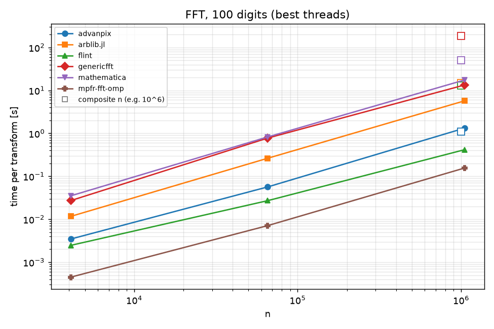
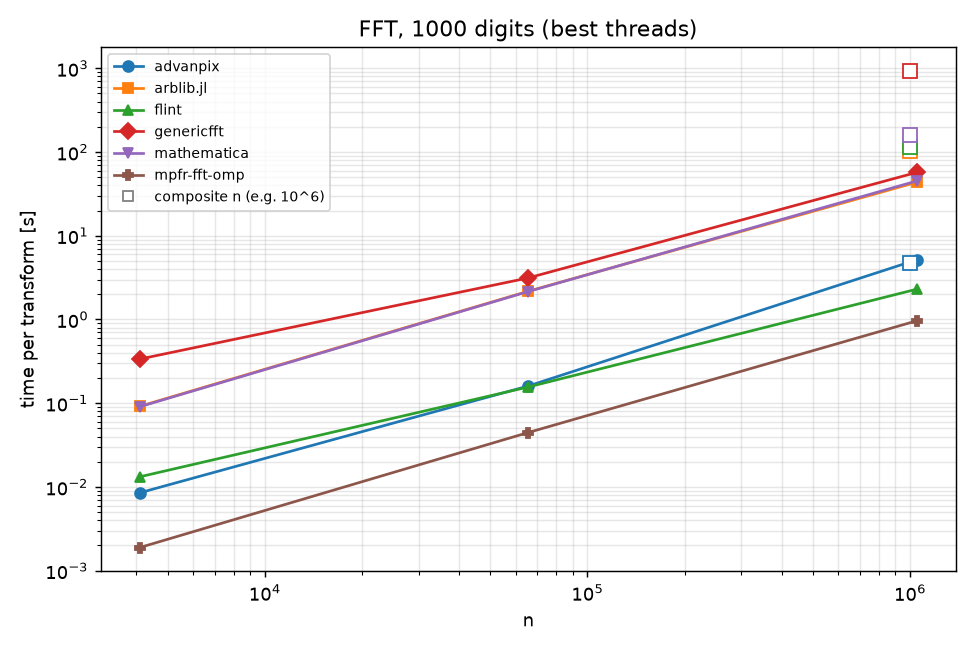
Time of one complex FFT (seconds), at the best thread count of each system; single-thread values in parentheses.

System	\(2^{20}\), 100 digits	\(2^{20}\), 1000 digits	\(10^{6}\), 1000 digits
Home-made OpenMP radix-2 (MPFR)	0.156 (5.1)	0.96 (41)	not supported
FLINT acb_dft	0.416	2.3 (50)	115
Advanpix fft	1.32	5.2 (59)	4.8
Arblib.jl	5.71	43.5	102
Mathematica Fourier	17.5	45	159
GenericFFT.jl	13.3	57	927

For power-of-two lengths the single-thread times are all close — home-made radix-2 41 s, Arblib 43 s, Mathematica 45 s, FLINT 50 s, Advanpix 59 s — and here too the cost of scalar operations dominates. Threads make the difference: the home-made implementation takes 0.96 s on 128 threads, FLINT 2.3 s, Advanpix 5.2 s. The butterflies within each stage of an FFT are independent, so even plain OpenMP wins as long as the threads actually work.

For the composite length \(10^6\) (\(= 2^6\cdot5^6\)) the picture reverses. Advanpix takes 4.8 s, on par with \(2^{20}\), but FLINT takes 115 s (50× its \(2^{20}\) time), Arblib 102 s, Mathematica 159 s, and GenericFFT 927 s; the non-power-of-two path of FLINT's acb_dft is effectively unusable. Arblib.jl's value equals FLINT's single-thread value because it is not threaded when called from Julia.

The practical guideline is simply "use power-of-two lengths; if that is impossible, use Advanpix".

7. Estimating the resources needed by Advanpix

To estimate the time and memory needed to actually run eigenvalue computations, I ran nonsymmetric diagonalizations for \(N=100\)–\(2000\) with Advanpix (64 threads), one point per process, recording the peak resident memory of the process (VmHWM in /proc/self/status).

N	100 digits, time	100 digits, peak RSS	1000 digits, time	1000 digits, peak RSS
300	5.7 s	0.8 GB	35 s	1.1 GB
500	17 s	1.0 GB	120 s	2.0 GB
1000	79 s	1.9 GB	12.4 min	6.1 GB
1500	3.8 min	3.3 GB	36 min	12.8 GB
2000	8.1 min	5.4 GB	80 min	22 GB

A power-law fit of the time gives \(N^{2.28}\) at 100 digits and \(N^{2.56}\) at 1000 digits, less than 3, but this is because the parallel efficiency improves with \(N\); once it saturates, the exponent returns to 3. For extrapolation I therefore also use a conservative formula with \(N^3\) anchored at the largest measured point.

\[ t(N, d) \approx 6.0\times10^{-7}\,\frac{d}{1000}\,N^3 \ \text{[s]} \quad (\text{64 threads, }100 \le d \le 1000) \]

The linearity in the number of digits \(d\) holds only within the range checked, 100–1000 digits (below it the fixed overhead dominates; above it the superlinear cost of multiplication kicks in).

Memory follows \(N^2\) closely, and separating the bytes per element from the 100- and 1000-digit coefficients gives

\[ M(N, d) \approx 0.7\ \text{GB} + N^2\,(700 + 4.7\,d)\ \text{[B]} \]

The fixed 700 B is the object overhead of MPFR / Advanpix, and the 4.7 B per digit is about 11× the theoretical mantissa size (0.415 B per digit), i.e. eig keeps working storage equivalent to roughly 10 input matrices.

From these, estimates for any \(N\) follow.

\(N\)	100 digits, time (fit / \(N^3\))	100 digits, memory	1000 digits, time (fit / \(N^3\))	1000 digits, memory
3000	18 min / 27 min	11 GB	3.5 h / 4.5 h	48 GB
5000	58 min / 2.1 h	29 GB	13 h / 21 h	132 GB
10000	4.7 h / 17 h	115 GB	3.2 days / 7 days	525 GB

\(N=10000\) at 1000 digits does not fit in the memory of this machine (512 GB). That memory becomes the limit before time does is an important point when choosing a machine.

The implications for choosing a machine: (1) the number of physical cores translates directly into speed (SMT is unnecessary, and better disabled); (2) the more digits, the more cores pay off; (3) handling \(N \ge 5000\) at 1000 digits needs at least 256 GB of memory, and \(N=10000\) needs 768 GB–1 TB; (4) the scaling of the matrix product is sensitive to memory bandwidth, so an 8-channel configuration (Threadripper PRO / EPYC class) is desirable — the question is how to secure the budget.

8. Summary by use case

Use case	Recommendation	Notes
Fast diagonalization of large matrices (many-core machine available)	Advanpix	Pin to physical cores. \(N=1000\) at 1000 digits in 12 min
Sequential, no license	GenericSchur (Julia), Eigen + mpreal, MPLAPACK	All within a factor of 2. MPLAPACK: GMP for 100 digits, MPFR for 1000. MPLAPACK has the edge for \(N \ge 1000\)
Certified eigenvalues	FLINT eig_multiple	\(N \le 100\) as a guide; fails for ill-conditioned matrices
32–64 digits suffice	MultiFloats (Julia)	30–40× faster than BigFloat
Many transcendental function calls	arb / Advanpix	4–6× faster than MPFR
FFT	Home-made OpenMP or FLINT for power-of-two lengths; Advanpix for composite lengths	Avoid FLINT for composite lengths
From Python	python-flint	mpmath is an order of magnitude slower
Avoid	cpp_bin_float (transcendentals), __float128 (speed), GenericFFT, Mathematica's Hermitian diagonalization

In the end, the time of arbitrary-precision linear algebra is determined by "how many scalar operations of 50 ns–1 µs each are called". Implementations differ by about 2×, and any further speedup comes only from parallelization. Among the candidates tested only Advanpix implements it; conversely, if parallel eigenvector computation were added to MPLAPACK or GenericSchur, they could compete on the same footing.

Appendix

A. Verification values

In every system the residual \(\max_k \|Av_k-\lambda_k v_k\|_\infty/(\|A\|_\infty\|v_k\|_\infty)\) was 1–2 digits below the target precision (\(10^{-99}\)–\(10^{-98}\) at 100 digits, \(10^{-300}\) or less at 1000 digits). MPLAPACK-GMP actually runs at 115 digits when 100 are requested, because the precision of mpf is rounded up to a multiple of 64 bits. The round-trip errors of the FFTs were likewise at the target precision.

B. Record of pitfalls

• Converting inputs from double precision shortens the mantissa and makes arb / MPFR multiplication appear faster than it is (Section 1).

• The Circus matrix is upper Hessenberg and the cost of Hessenberg reduction is not included (Sections 1 and 5).

• The GMP backend of MPLAPACK 3.0 ignores mpf_set_default_prec; the precision must be set with gmpxx::set_default_mpf_precision_bits (if this goes unnoticed, the default 512 bits stays fixed and the 100- and 1000-digit runs take the same time).

• Advanpix becomes more than 5× slower when SMT threads are used (Section 4).

• FLINT's certified eigenvalues take an explosive amount of time on ill-conditioned matrices (3.3 hours at 1000 digits, \(N=300\)).

C. Code and data

mpbench contains the complete set of programs and results used for this article. mpbench/readme describes how to build and run them (in Japanese). mpbench/env.txt records the CPU, memory, kernel, compiler, and library versions. mpbench/results.csv and mpbench/advanpix_scaling.csv contain the measurements.